
Exploring Different Types of Distributions for Sampling

In statistics, sampling serves as the bedrock for drawing meaningful inferences about an entire population without the prohibitive cost, time, and logistics of surveying every single member. Whether investigating citizen demographics across a nation, defect rates along an industrial manufacturing line, or millions of digital financial transactions, examining every unit is rarely feasible. Instead, researchers rely on a carefully gathered subset—a sample—to uncover the characteristics of the larger whole.
To ensure that findings are reliable, the sample must be truly representative of its parent population. Evaluating how data points fall across a spectrum reveals the sample's underlying probability distribution. By mapping which outcomes occur frequently, which appear rarely, and how much variability exists, researchers can determine whether their sample accurately mirrors the target population and select the appropriate mathematical tools for deeper inquiry.
Key takeaways
- Probability distributions illustrate the frequency, spread, and variability of discrete counts and continuous measurements within a sample.
- Theoretical models like normal, uniform, binomial, Poisson, exponential, and gamma distributions provide mathematical foundations for real-world phenomena.
- Differentiating between discrete count data and continuous duration measurements prevents fundamental errors in probability estimation.
- When empirical sample data diverges significantly from standard parametric models, researchers must utilize non-parametric methods to avoid biased deductions.
Core probability distributions in statistical sampling
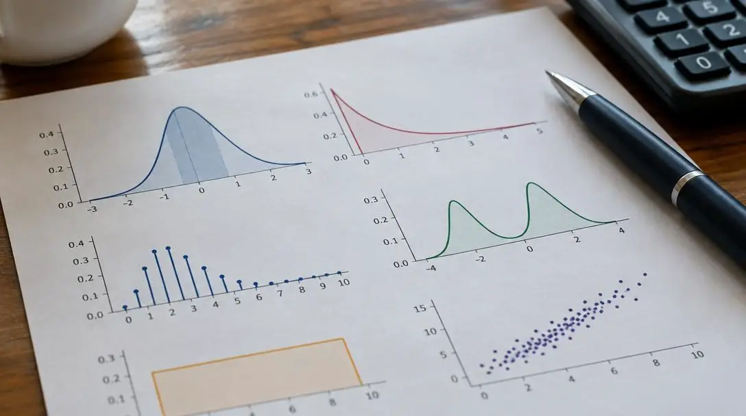
Probability distributions are broadly split between discrete distributions, which handle distinct values such as integer counts, and continuous distributions, which capture values along an unbroken continuum. Recognizing the exact nature of observed data guides analysts toward the appropriate mathematical model.
Normal distribution
The normal distribution stands as one of the most widely applied theoretical models in statistics. Visually recognized as a symmetrical bell curve, it frequently describes natural physical characteristics, standardized academic test scores, and systemic measurement errors. The location and geometric spread of the curve are governed entirely by two measures: the mean, which marks the central peak, and the standard deviation, which sets the width of the bell.
A central feature of the normal distribution is the empirical 68-95-99.7 rule. Under this benchmark, approximately 68% of all observed data points sit within one standard deviation of the mean, 95% fall within two standard deviations, and 99.7% reside within three standard deviations. Because of this predictable structural dispersion, the normal distribution serves as the primary baseline for a vast array of parametric statistical analyses.
Uniform distribution
A uniform distribution emerges when every outcome within an established range possesses an identical probability of occurring. Rather than producing a distinct peak or tapering tails, the probability density remains flat across the entire interval of interest. A classic example is flipping a fair coin, where the likelihood of heads or tails is balanced equally at 0.5.
Because it offers an impartial spread where no single outcome is favored, the uniform distribution plays a vital role in computer modeling, algorithmic simulations, and Monte Carlo methods. In these computational frameworks, generating unbiased random numbers across fixed boundaries forms the baseline requirement for simulating complex, multi-stage processes.
Binomial distribution
The binomial distribution models scenarios defined by a fixed sequence of independent trials, where each trial yields a binary outcome: success or failure. The distribution is mathematically defined by three primary elements: the total number of trials conducted, the baseline probability of success on any single trial, and the observed tally of successful events.
Tossing a coin a set number of times—such as recording the number of heads across ten flips—represents a standard binomial process. Outside of theoretical examples, the binomial distribution is routinely employed in industrial quality control routines, binary clinical research trials, and public opinion polling based on yes-or-no survey questions.
Poisson distribution
The Poisson distribution models the likelihood of a specific count of events taking place within a predetermined boundary of time or physical space. This distribution operates under the core assumption that individual events occur independently and at a constant average rate. Unlike models constrained by a predetermined total number of trials, the Poisson model requires only a single governing parameter: the average rate of occurrence.
Fields such as engineering, finance, and biology rely heavily on Poisson modeling to quantify relatively rare occurrences. Common applications include tracking equipment breakdowns in an industrial facility, recording vehicular collisions at a specific intersection, or assessing system defects. While there is no theoretical ceiling on the number of events that might happen, extremely elevated counts become mathematically improbable.
Exponential distribution
While the Poisson distribution focuses on the total number of occurrences within an interval, the exponential distribution models the continuous duration of time that elapses between two successive, independent events occurring at a constant rate. Governed by a single rate parameter, this continuous distribution determines the expected waiting time until the next event takes place.
In operational settings, the exponential model is used to track customer arrival intervals at retail counters, queues at service kiosks, or the operational lifespan between equipment malfunctions on a production floor. It is closely tied to Poisson processes, translating count-based arrival dynamics into continuous time intervals.
Gamma distribution
The gamma distribution constitutes a broad family of continuous probability distributions that serves as a generalized extension of the exponential distribution. Whereas the exponential model evaluates the wait time until a single event occurs, the gamma distribution accommodates more complex scenarios involving multiple stages, accumulated operational wear, or compound waiting durations.
Characterized by two distinct parameters—the shape parameter and the scale parameter—the gamma distribution offers exceptional structural flexibility. By modifying these two inputs, analysts can model diverse levels of skewness and dispersion, making it a powerful tool for analyzing intricate industrial systems, hydrological precipitation patterns, and multi-tiered operational workflows.
Comparative attributes of sampling distributions
Selecting the correct statistical model requires matching empirical observations with theoretical properties. The following table highlights the operational distinctions, parameter requirements, and real-world applications across standard probability distributions.
| Distribution | Data Type | Key Parameters | Defining Characteristic | Common Practical Applications |
|---|---|---|---|---|
| Normal | Continuous | Mean, Standard Deviation | Symmetric bell curve; follows the 68-95-99.7 rule | Human heights, standardized test results, measurement errors |
| Uniform | Discrete or Continuous | Interval boundaries (minimum, maximum) | Equal probability for all outcomes across the range | Coin flips, Monte Carlo simulations, randomized trial inputs |
| Binomial | Discrete | Number of trials, Probability of success | Fixed count of independent binary trials (success/failure) | Quality assurance, yes-or-no surveys, clinical trials |
| Poisson | Discrete | Average rate of occurrence | Counts occurrences over a fixed time or space interval | Equipment failures, intersection accidents, rare biological mutations |
| Exponential | Continuous | Rate parameter | Models continuous duration or wait time between events | Customer queue intervals, machine lifespans between breakdowns |
| Gamma | Continuous | Shape parameter, Scale parameter | Flexible skewness; generalizes waiting times across multi-stage processes | Complex system queues, accumulated service stages, environmental modeling |
Evaluating the pattern of outcomes observed in our sample reveals whether our data reflects the anticipated structure of the target population.
How distribution analysis operates in practice
Moving from raw data collection to mathematical modeling requires a systematic process. Analysts assess empirical observations through a sequence of analytical procedures designed to verify compatibility with theoretical distributions.

The workflow begins with data collection, wherein researchers gather sample units from the parent population using sound sampling strategies designed to minimize bias. Once recorded, the data undergoes initial visualization through frequency plots or histograms. These graphical representations reveal the underlying shape, spread, central tendencies, and potential skewness present within the observations.
Next, analysts proceed to summary calculation, computing fundamental metrics such as the sample mean, variance, standard deviation, and event counts. These figures inform the model matching phase, during which the empirical data is evaluated against candidate theoretical profiles to determine whether a continuous or discrete framework is warranted.
When a plausible distribution is identified, researchers initiate parameter estimation, calculating the exact metrics that define that curve—such as the mean and standard deviation for a normal model, the rate parameter for a Poisson or exponential model, or the shape and scale inputs for a gamma distribution. Finally, goodness-of-fit evaluation applies formal statistical tests to compare observed sample frequencies against expected theoretical values, confirming whether the mathematical distribution matches the real-world sample.
Step-by-step framework for identifying sample distributions
Determining the correct distribution for an empirical dataset requires methodical validation. Practitioners utilize the following structured steps to categorize their sample data accurately.
- Define the population and variable type: Identify the target population under study and clarify whether the primary metric is discrete (such as counts of distinct occurrences) or continuous (such as measurements of time, weight, or length).
- Collect a representative sample: Extract observations using standardized sampling protocols that preserve event independence and minimize systematic collection bias.
- Tabulate and plot the sample: Generate histograms, empirical density curves, or frequency tables to visually inspect the distribution's shape for symmetry, skewness, flat profiles, or discrete clusters.
- Calculate descriptive parameters: Derive basic sample metrics, including the sample mean, dispersion metrics like the standard deviation, and observed rate parameters.
- Evaluate against distribution criteria: Assess whether data values align with theoretical benchmarks. Verify whether the sample conforms to the 68-95-99.7 rule for normality, displays constant probability for a uniform model, represents fixed binary trials for a binomial model, captures independent counts for a Poisson model, or reflects continuous intervals for an exponential or gamma model.
- Decide on the analytical approach: If the empirical data satisfies the requirements of a theoretical distribution, apply the corresponding parametric analytical methods. If the sample deviates significantly from known distributions, adopt non-parametric techniques that do not rely on distributional assumptions.
Critical mistakes to avoid in distribution analysis
Misinterpreting probability distributions can distort research findings, leading to flawed conclusions and incorrect forecasts. Analysts should watch out for several recurring analytical traps when handling sample data.
- Assuming normality by default: While human physical traits and standardized test scores often form a symmetric bell curve, many operational datasets—such as waiting intervals, binary choices, and rare events—exhibit heavy skewness or bounded ranges that violate normality assumptions.
- Confusing discrete counts with continuous intervals: Attempting to fit continuous models to discrete counts, such as coin tosses or defect tallies, generates inaccurate probability calculations.
- Mixing up Poisson and exponential applications: While both frameworks rely on independent events occurring at a constant rate, confusing the count of events within a fixed period (Poisson) with the time elapsed between those events (exponential) leads to misapplied formulas.
- Ignoring independence requirements: Binomial, Poisson, and exponential models collapse if individual observations influence one another. When events cluster or correlate, assuming independence produces biased statistical inferences.
- Overlooking the 68-95-99.7 rule: Applying standard normal dispersion percentages to asymmetric, heavily skewed, or multimodal datasets produces distorted estimates of data clustering around the mean.
- Forcing data into theoretical models: When collected samples fail standard goodness-of-fit assessments, researchers must resist the temptation to force the data into a standard distribution, turning instead to non-parametric procedures.
Frequently asked questions
What is the difference between a discrete and a continuous distribution?
A discrete distribution models distinct, separate values such as whole integer counts of events, coin tosses, or survey responses. A continuous distribution models measurements that can take on any fractional value along an uninterrupted spectrum, such as time durations, heights, and weights.
How do the Poisson and exponential distributions differ if both rely on a constant rate?
The Poisson distribution measures the discrete number of times an event occurs within a designated window of time or space. The exponential distribution measures the continuous duration of time that elapses between those individual occurrences.
What should you do if your sample data does not fit any standard distribution?
When empirical data fails goodness-of-fit evaluations and cannot be accurately described by a standard distribution, analysts should use non-parametric statistical methods, which perform valid statistical evaluations without making rigid distributional assumptions.
Why is the 68-95-99.7 rule important in sampling?
The 68-95-99.7 rule establishes the baseline spread of data within a normal distribution, dictating that roughly 68%, 95%, and 99.7% of values fall within one, two, and three standard deviations from the mean, respectively. This predictable dispersion provides a core benchmark for evaluating parametric consistency.
When is a uniform distribution preferred over a normal distribution?
A uniform distribution is preferred when every outcome across a bounded range has an equal likelihood of occurring, making it foundational for Monte Carlo computational algorithms, randomized trials, and simulation modeling where no central tendency should exist.
The bottom line
Understanding probability distributions provides the essential framework for valid statistical deduction. When sampling from an expansive population, researchers must ascertain whether their collected data reflects the anticipated mathematical structure of that population. Each distribution family carries distinct structural characteristics, parameter constraints, and analytical requirements.
By properly categorizing whether data represents discrete event counts, continuous durations, or symmetrical variations around a central mean, analysts can select the correct tools for their investigations. Whether modeling equipment lifespans through exponential curves, analyzing rare industrial accidents with Poisson processes, or adopting non-parametric alternatives when data resists standard categorization, identifying the true distribution ensures that subsequent inferences remain methodologically sound.